Part A: The Power of Diffusion Models!
Overview
In this part, I tried to implement diffusion sampling loops, and use them for other tasks such as inpainting and creating optical illusions.
Sampling Loops
1.0: Setup
In this part, I set up the environment and load the necessary libraries and models. Download the precomputed Text embedding model and the pretrained diffusion model. And try sampling from the diffusion model with seed 180. Output images are shown below.


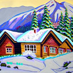
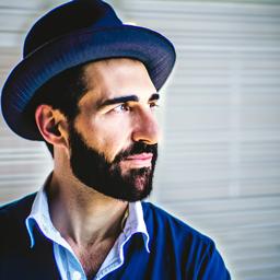
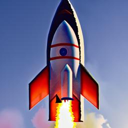
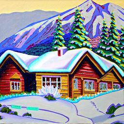
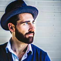

As we can see, the model can generate a wide variety of images, from oil paintings to rocket ships base on the prompt_embeds, and the images are generated in two stages. The first stage generates a rough sketch of the image, while the second stage refines the sketch to create a more detailed image. And num_inference_steps is the number of steps to run the model for each stage. The higher the number, the more detailed and smoother the image will be.
1.1 Implementing the Forward Process
In this part, we implement the forward process of the diffusion model. Start with a clean image, we add noise to it at each time step to create a noisy image based on the equation: \( x_t = \sqrt{\bar{\alpha}_t} x_0 + \sqrt{1 - \bar{\alpha}_t} \epsilon \quad \text{where}~ \epsilon \sim N(0, 1) \tag{2} \)
We use alphas_cumprod variable that include an array of hyperaparameters, and alphas_cumprod[t] is the value of \( \bar{\alpha}_t \) at timestep t.
Outputs


1.2: Classical Denoising
After implementing the forward process, I use classical denoising methods to denoise the images. First take noise image for timesteps [250,500,750], use Gaussian blur to denoise the images. The resulte is shown below.


1.3 One-Step Denoising
In this step, UNet is used to denoise images by first identifying and recovering the Gaussian noise present and then removing it to approximate the original, noise-free image. Since the diffusion model uses text conditioning, we can use the prompt_embeds = "a high quality photo" to guide the denoising process. The result is shown below.


1.4: Iterative Denoising
Denoising UNet does better than classical denoising methods. To get a better result, I use iterative denoising. We start with a noisy image \( x_{1000} \) at timestep 1000. Normally, we would denoise this step-by-step—going from \( x_{1000} \) to \( x_{999} \), then \( x_{998} \), and so forth. However, this approach can be slow and computationally intensive. One way to reduce the time is to create a list of timesteps called `strided_timesteps` that skips certain steps. This allows us to apply the diffusion model at specific intervals, making the denoising process more efficient.
The iterative denoising process can be described by the following equation: \[ x_{t'} = \frac{\sqrt{\bar{\alpha}_{t'}}\beta_t}{1 - \bar{\alpha}_t} x_0 + \frac{\sqrt{\alpha_t}(1 - \bar{\alpha}_{t'})}{1 - \bar{\alpha}_t} x_t + v_\sigma \tag{3} \]
Here, \( x_t \) is the image at timestep \( t \), and \( x_{t'} \) is the denoised image at timestep \( t' \). By using this equation, we can gradually reduce noise at each selected timestep, efficiently bringing the image closer to its original form.


1.5 Diffusion Model Sampling
In previous sections, we used the diffusion model to denoise images. Now, we will use the model to generate new images by setting i_start = 0. Means start from a pure noise image, and generate images based on the prompt_embeds = "a high quality photo".


1.6 Classifier-Free Guidance (CFG)
Some of the images generated by Diffusion Model are meaning less, to improve the image quality, we can use Classifier-Free Guidance (CFG) to guide the sampling process. Basically, we compute the conditional nosie and unconditional noise, sum them with a scaling factor(7), and use the result to guide the sampling process. Output images are shown below.


1.7 Image-to-image Translation
By applying a small amount of noise initially, the denoised image will closely resemble the original, enabling subtle edits. This iterative process, guided by the SDEdit algorithm, gradually refines the image back towards its original state, allowing for controlled modifications. Next, we will experiment with different levels of noise by using starting indices of [1, 3, 5, 7, 10, 20]. This will produce a series of progressively "edited" images, with each step bringing the noisy image closer to its original form. The resulting output images are displayed below.


If we start from some unrealistic images, the denoising process will help us turn it to a more realistic image. Output images are shown below.


1.7.2 inpainting
In this part, I use the diffusion model to inpaint images. I start with a clean image, and mask out a portion of the image. Then, I use the diffusion model to inpaint the masked region. The result is shown below.


1.7.3 Text-Conditioned Image-to-image Translation
In this part, I use the diffusion model to perform text-conditioned image-to-image translation. I start with a clean image, add some noise, and use the prompt_embeds = "a high quality photo" to guide the translation process. The result is shown below.


1.8 Visual Anagrams
In this part, we start with a imaage x_t at step t, with promot "an oil painting of an old man", to get the noise, also, flip the image upside down denoise with different promote "an oil painting of people around a campfire", then flip the image back to get the noise estimate. algorithm and ouput images are shown below.
\( \epsilon_1 = \text{UNet}(x_t, t, p_1) \)
\( \epsilon_2 = \text{flip}(\text{UNet}(\text{flip}(x_t), t, p_2)) \)
\( \epsilon = (\epsilon_1 + \epsilon_2) / 2 \)


1.9 Hybrid Images
Similar to the previous part, we start with an image \( x_t \) at step \( t \), using the prompt "a lithograph of waterfalls" for high-frequency noise and "a blurry photo of a skull" for low-frequency noise.
Here is the algorithm:
\( \epsilon_1 = \text{UNet}(x_t, t, p_1) \)
\( \epsilon_2 = \text{UNet}(x_t, t, p_2) \)
\( \epsilon = f_{\text{lowpass}}(\epsilon_1) + f_{\text{highpass}}(\epsilon_2) \)


Part 2: Training a Diffusion Model on MNIST
In this part, we will train own diffusion model on MNIST
Part 1: Training a Single-Step Denoising UNet
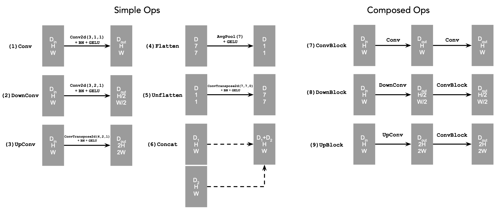
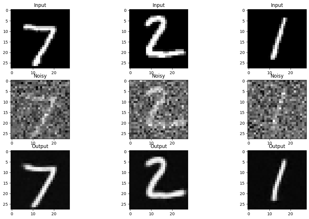
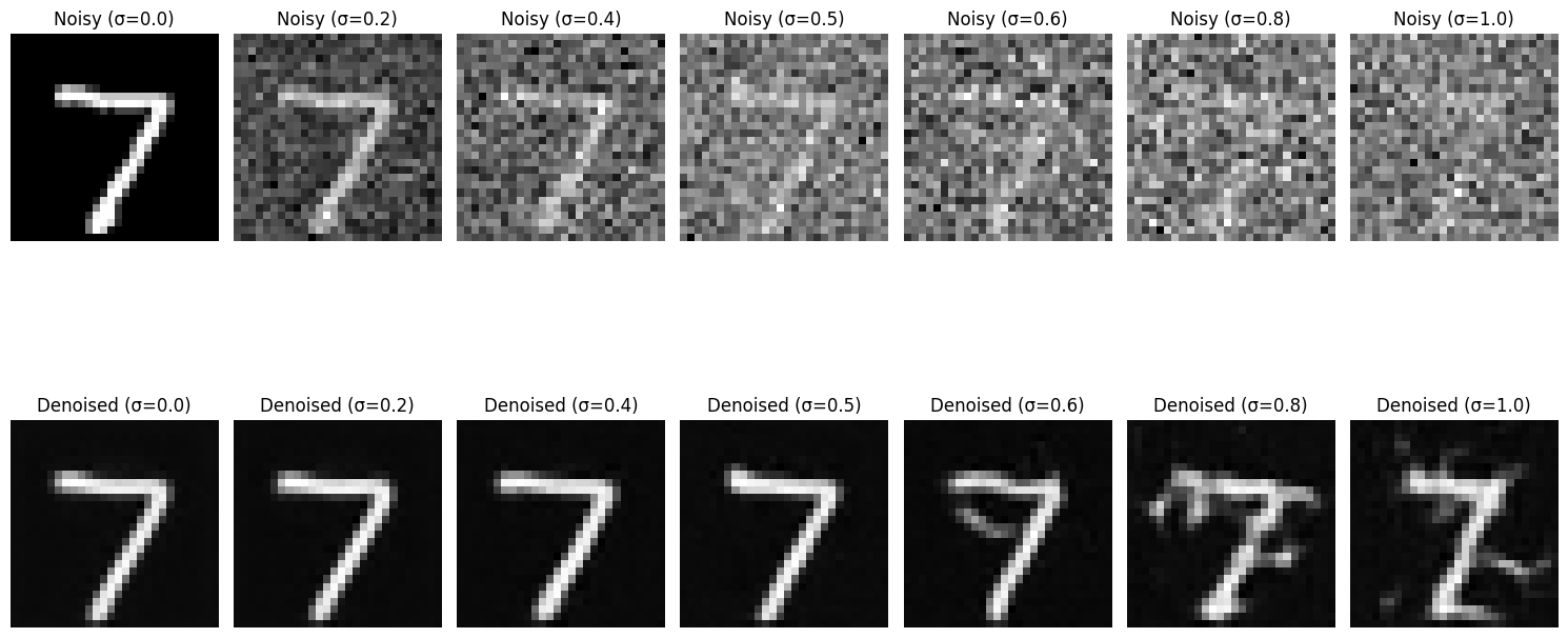
In this part, we will first train a single-step denoising UNet on the MNIST dataset. The model will take a noisy image as input and output a denoised image, optimize over an L2 loss. Follow by the Unet model below:
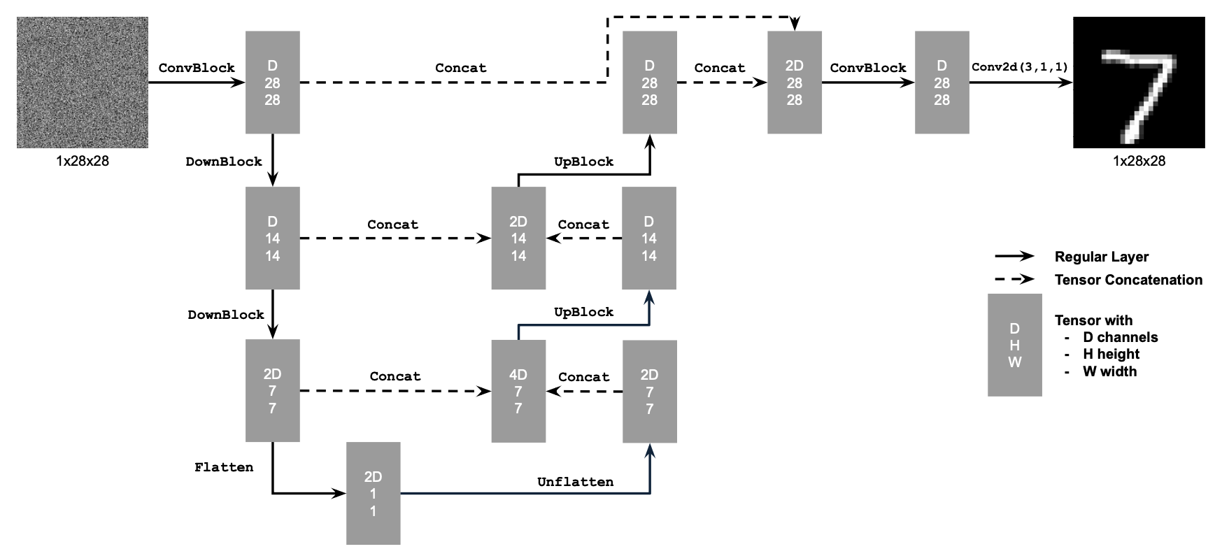
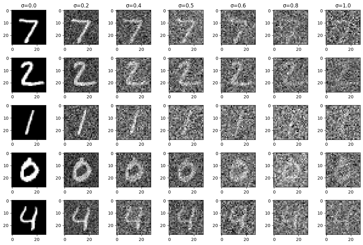
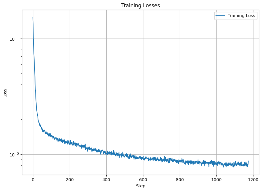
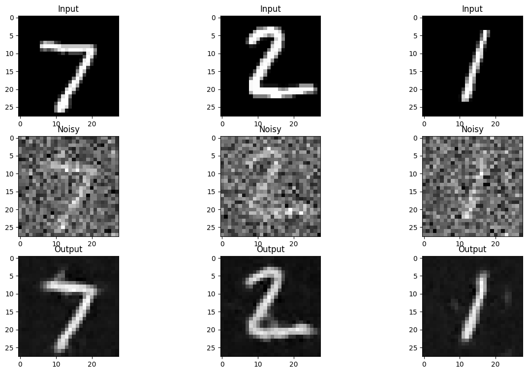
The different noise level for MNIST digits, training curve, and traning resulte are shown below.
Part 2: Training a Diffusion Model on MNIST
In this part, we will training a UNet model iteratively denoise an image, and implement the Denoising Diffusion Probabilistic Models
(DDPM) on the MNIST dataset.
Start with the first change, we use the UNet to pridect teh added noise instead of teh clean img.
Follow the loss function here: \[L = \mathbb{E}_{\epsilon,z} \|\epsilon_{\theta}(z) - \epsilon\|^2 \tag{B.3}\]
And generate noisy images for some timestep, \[x_t = \sqrt{\bar\alpha_t} x_0 + \sqrt{1 - \bar\alpha_t} \epsilon
\quad \text{where}~ \epsilon \sim N(0, 1). \tag{B.4}\]
Also, add the time conditioning to the UNet model like this:


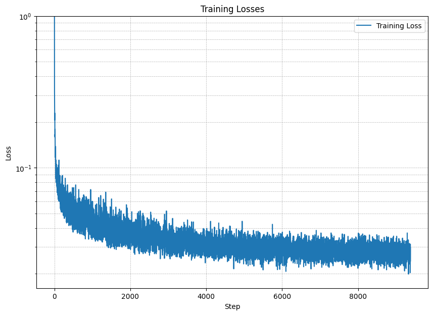
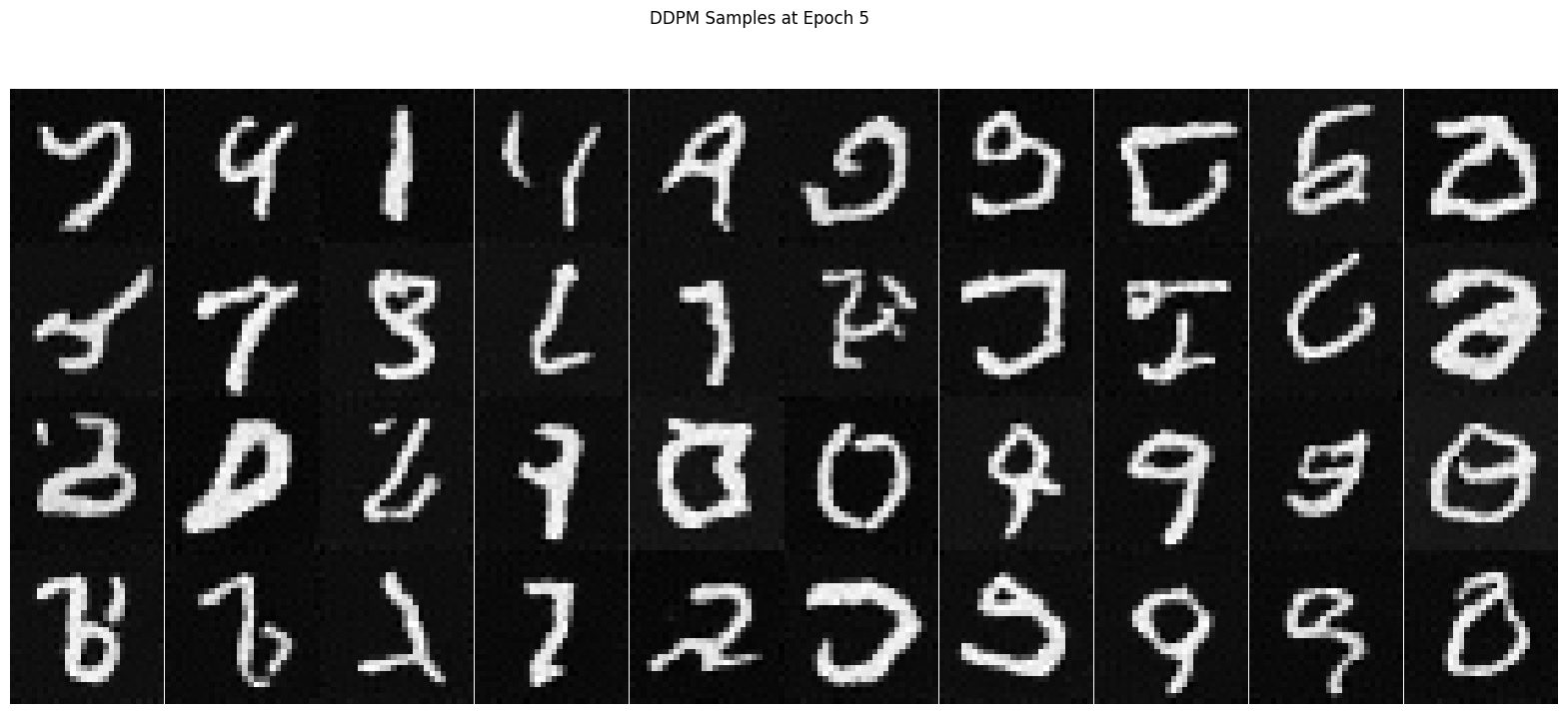
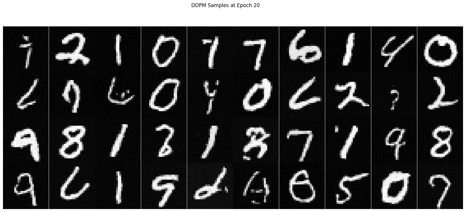
Below are the algorithm for Sampling and training time conditioned UNet, training curve and the training results.

2.4 Adding Class-Conditioning to UNet
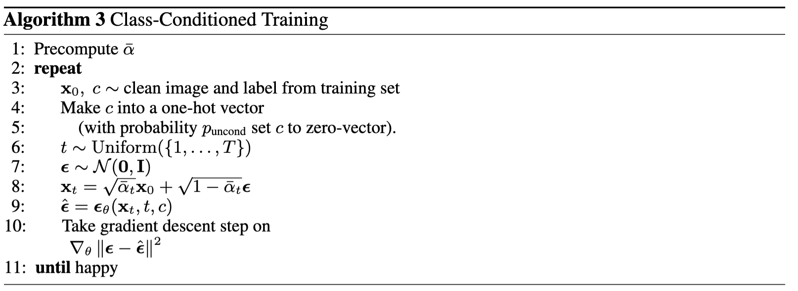
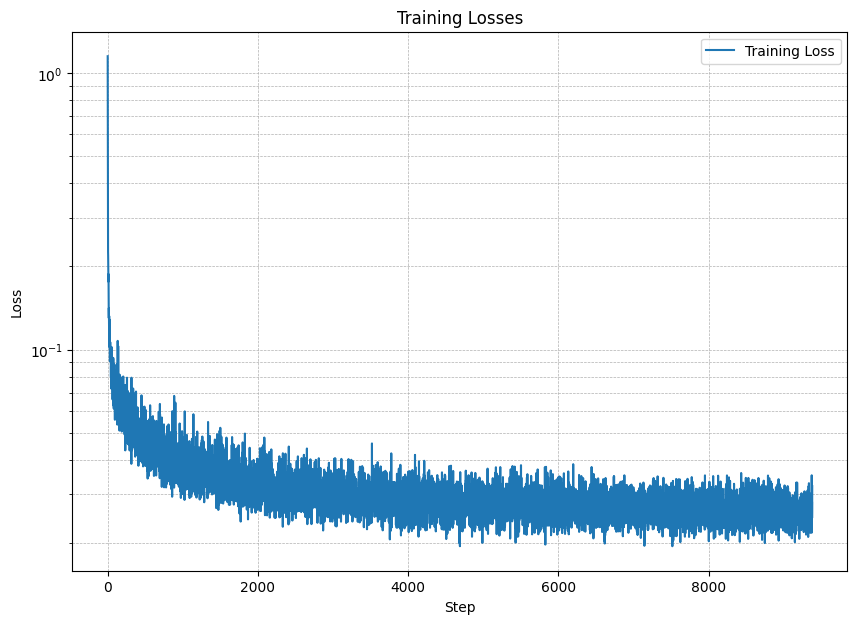
In this part, we will add class-conditioning to the UNet model. The model will take a noisy image and a class label as input and output a denoised image. The class label will be used to condition the model on the class of the digit in the image. The loss function is defined as: \[ L = \mathbb{E}_{\epsilon,z} \|\epsilon_{\theta}(x_t,t, c) - \epsilon\|^2 \tag{B.5} \] The algorithm for training the class-conditioned UNet and loss curve are shown below:
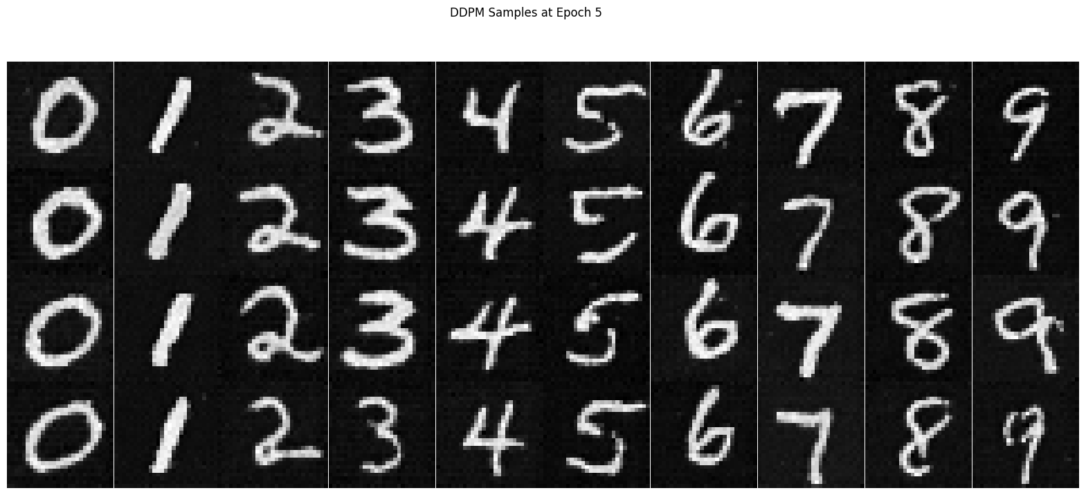
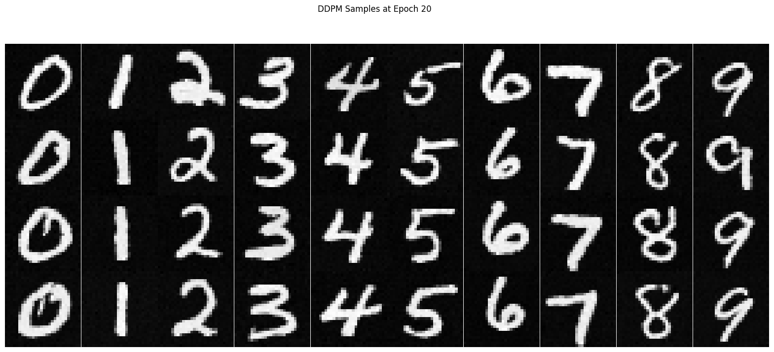
The sampling process are Similar to part A, and we are using classifier-free guidance to guide the sampling process.\[\gamma = 5.0\] The output images are shown below.
