Part A. IMAGE WARPING and MOSAICING
Overview
For part A, I first take pictures at fixed points with different angles and use the provided tool to get the corresponding points of the images.
Then, I calculate the homography matrix using the function computeH(im1_pts, im2_pts) and warp the image using the function warpImage(img, H).
Finally, I blend the images together to get the final result.
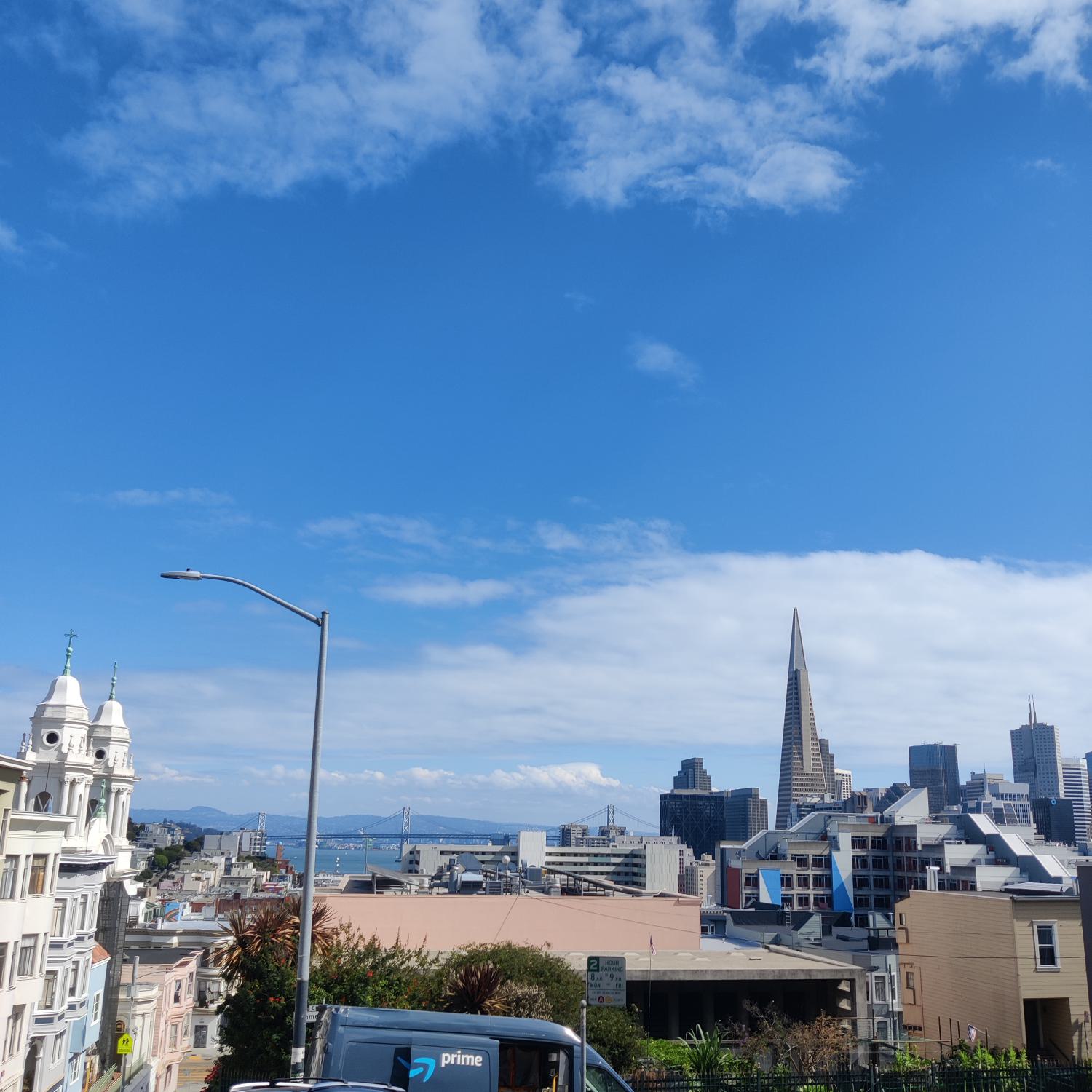
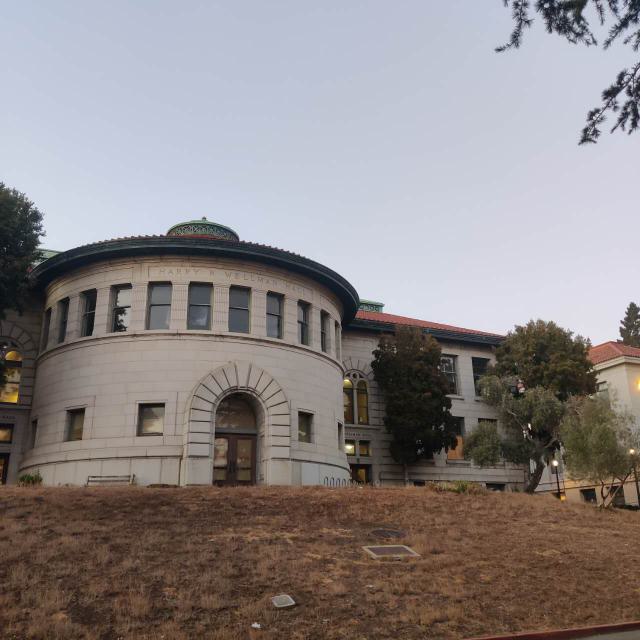
Shoot and digitize pictures
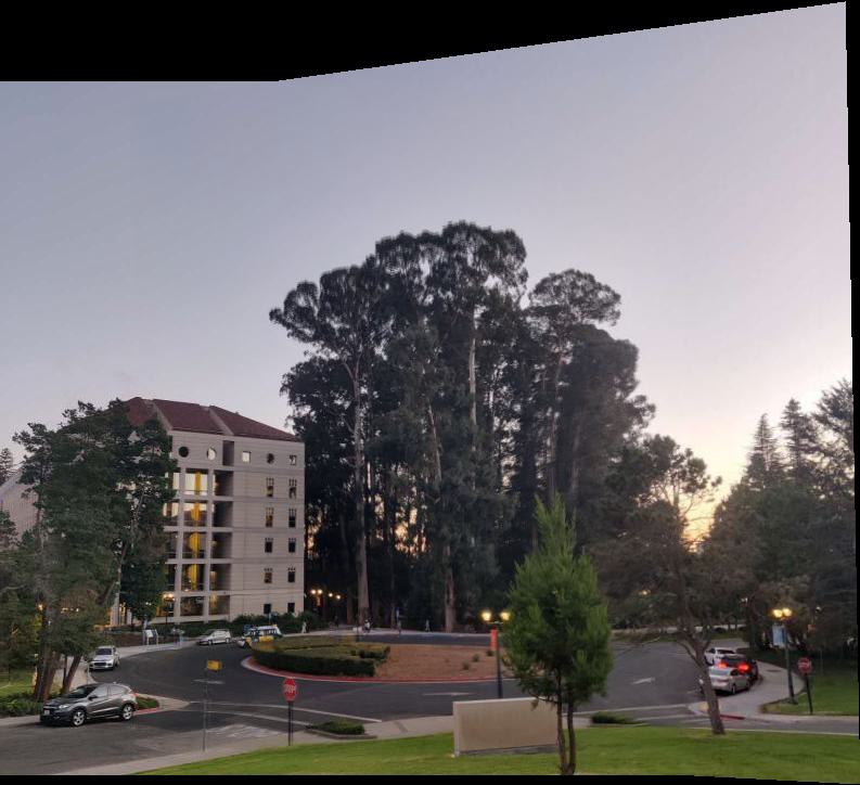
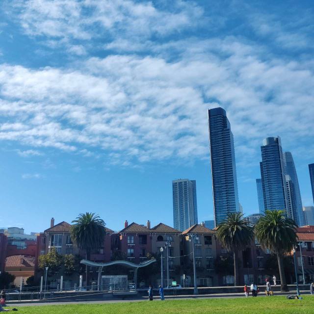
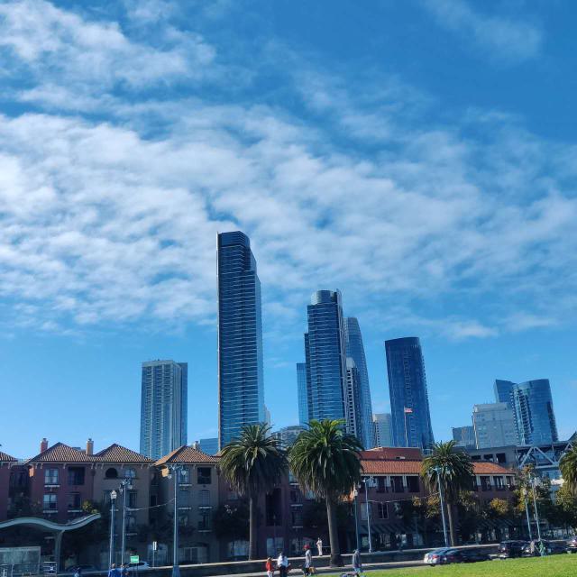
Take pictures at fixed points with different angles, and digitize the images.
Recover homographies
Use the provided tool to get the corresponding points of the images, then calculate the homography matrix using the function computeH(im1_pts, im2_pts).
For each pair of corresponding points $(x, y)$ from image 1 and $(x', y')$ from image 2, we construct the following matrix equation to solve for the homography matrix:
$$\begin{bmatrix} wx' \\ wy' \\ w \end{bmatrix} = H \cdot \begin{bmatrix} x \\ y \\ 1 \end{bmatrix}$$
$$\begin{bmatrix} wx' \\ wy' \\ w \end{bmatrix} = \begin{bmatrix} a & b & c \\ d & e & f \\ g & h & 1 \end{bmatrix} \begin{bmatrix} x \\ y \\ 1 \end{bmatrix}$$
Simplifying gives:
$$ x' = \frac{ax + by + c}{gx + hy + 1}, \quad y' = \frac{dx + ey + f}{gx + hy + 1} $$
Rearranging, we get two linear equations:
$$ ax + by + c -gx \cdot x' - hy \cdot x' = x' $$
$$ dx + ey + f - gx \cdot y' - hy \cdot y' = y' $$
This results in the matrix form:
$$ \begin{bmatrix} x & y & 1 & 0 & 0 & 0 & -x \cdot x' & -y \cdot x' \\ 0 & 0 & 0 & x & y & 1 & -x \cdot y' & -y \cdot y' \end{bmatrix} \cdot \begin{bmatrix} a \\ b \\ c \\ d \\ e \\ f \\ g \\ h \end{bmatrix} = \begin{bmatrix} x' \\ y' \end{bmatrix}$$
Then, apply least squares to solve for the homography matrix.
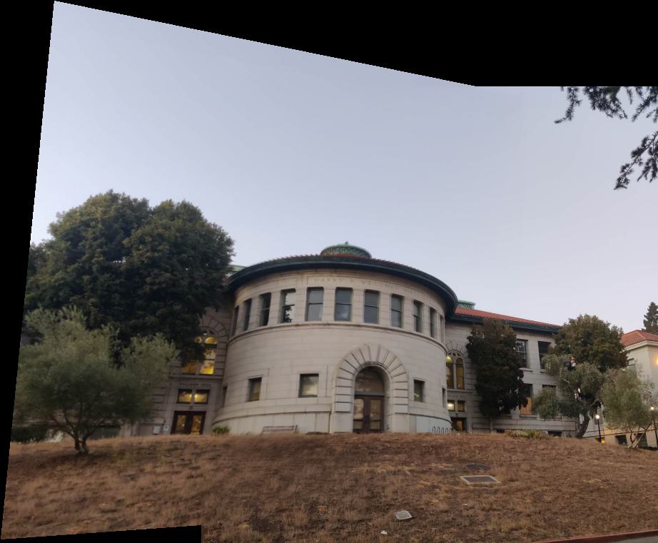
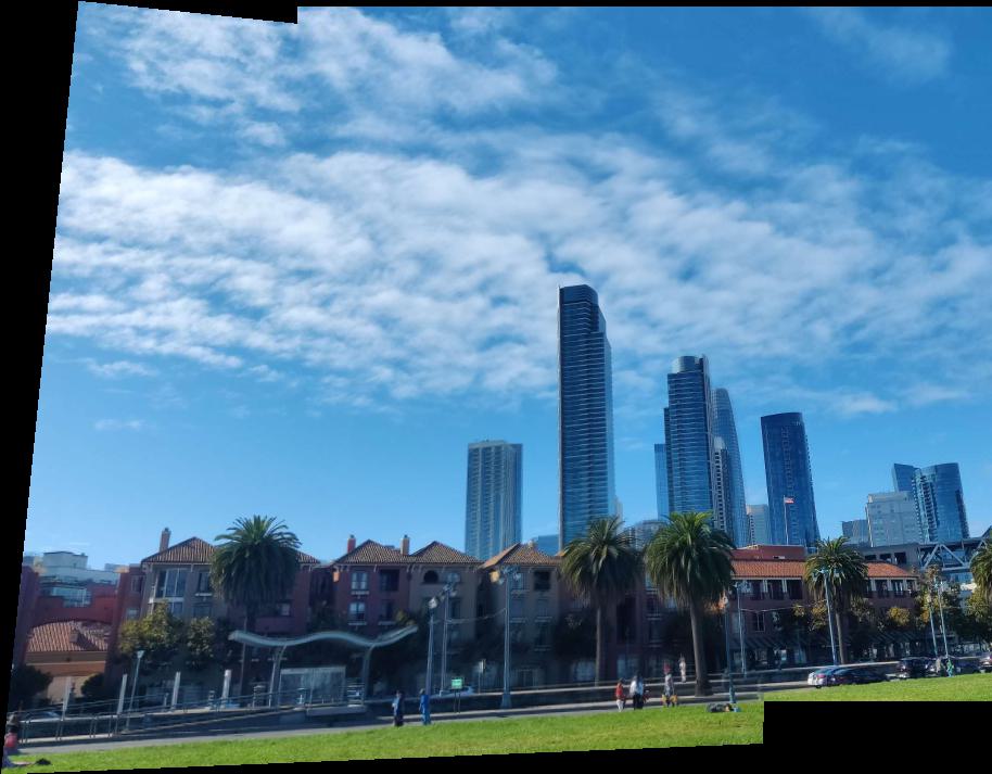
Warp the image
To warp the image, use the function warpImage(img, H).
First, I calculate the shape of the output image using the four corners of the original image multiplied by the homography matrix $H$.
Normailize the calculated bounds, then create a 2D grid of coordinates for the output image and map it back to the input image using the inverse of $H$.
The griddata function is used, it takes the input image coordinates, the pixel values from the input image (reshaped into a 1D array), and the back-projected coordinates xi.
And returns the interpolated pixel values for the warped image, then reshape it back to the output image shape.
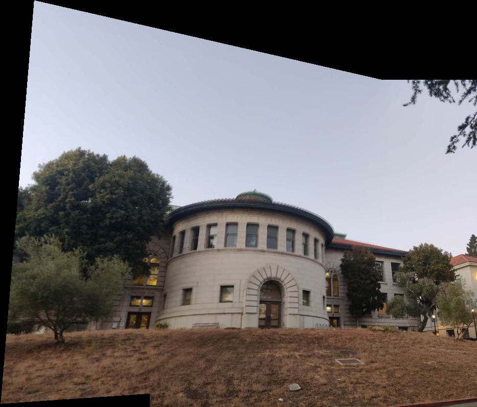
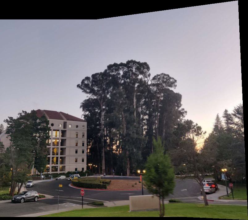
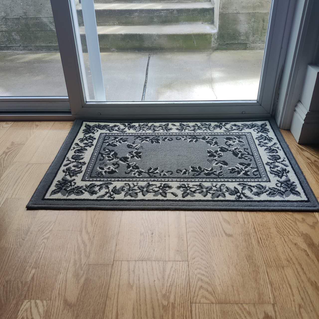
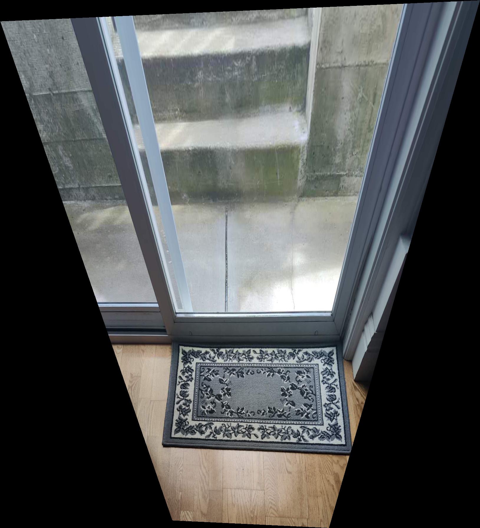
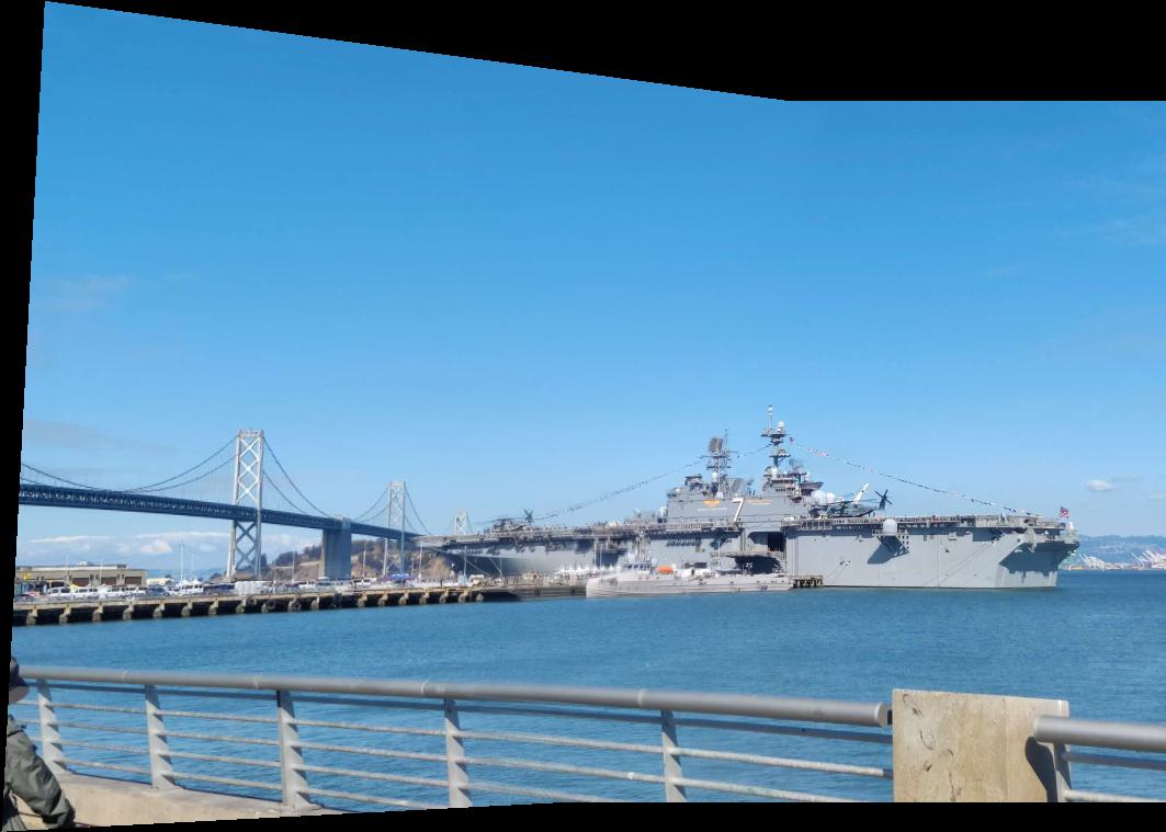
Outputs
Blend the images
After the warpImage function works correctly, we can merge two images taken from the same position but at different angles into a single combined
image. To blend the two images, the following steps are taken:
Workflow
- The first way I tried is creating a mask with values of either 1 or 0.5. This is a straightforward blending method where non-overlapping regions of the images are given full weight (mask value = 1), and overlapping regions are blended with half weight (mask value = 0.5).
- It not works well enough then I blend the images based on the distance of each pixel from the edge of the non-overlapping areas(Use function
cv.distanceTransform(mask1, cv.DIST_L2, 5)), which give me a smoother transition between the images.
Outputs


Part B.FEATURE MATCHING for AUTOSTITCHING
Overview
For part B, we will implement a auto mathcing function to find the corresponding points of the images
base on paper “Multi-Image Matching using Multi-Scale Oriented Patches” but with several simplifications
Then base on the homography matrix, we warp the image using the function warpImage(img, H).
Finally, we will blend the images together to get the final result.
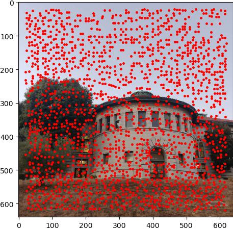
Harris Interest Point Detector
The Harris Interest point detector is used to detect the interest points in the image. It basically caculate the gradient of the image and then caculate the matrix M for each pixel, base on the eigenvalues of M, we can determine if the pixel is a interest point. I used the code provide by project website harris.py.
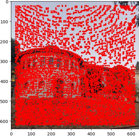
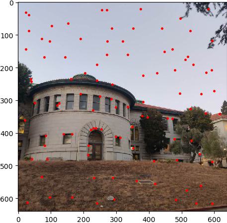
Implement Adaptive Non-Maximal Suppression
we already get the interest points, but there is so many points in the image, we need to reduce the number of points to make the matching process faster. One way to do this is to implement Adaptive Non-Maximal Suppression, which is a method to reduce the number of interest points by selecting only the most important ones. base on the equaction form the paper, \( r_i = \min_j \left| x_i - x_j \right|, \text{ s.t. } f(x_i) < c_{\text{robust}} f(x_j), \ x_j \in \mathcal{I} \) For every point \( x_i \) in the interest points, we caculate the distance to the nearest point \( x_j \) that has a higher score than \( x_i \), and find the min distance \( r_i \) for each point. Then we sort the points by the value of r_i, and select the top \( N \) points as the final interest points. I select crobust = 0.9 as described in the paper.

Implement Feature Descriptor extraction
After we get the interest points, we need to extract the feature descriptor for each point. As the paper mentioned, we use the 40x40 window around the interest point as the feature descriptor, apply low pass filiter, and then downsample the window to 8x8.


Implement Feature Matching
After we get the feature descriptor for each point, we need to match the points between two images.
For each point in the first image, we caculate the distance to all the points in the second image,
and select the point with the smallest distance as the corresponding point, use lowe ratio to filter the points.
If the min and second min distance is too close, we will ignore this point.
Then, apply the same process for the second image, and caculate the distance for each point in the second image to the first image.
If the distance is the same as the distance caculated in the first step, we will add this point to the matching points.
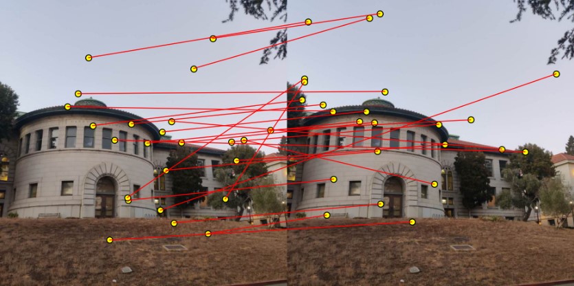
Although the feature matching works for most of the points, there are still some points that are not matched correctly.
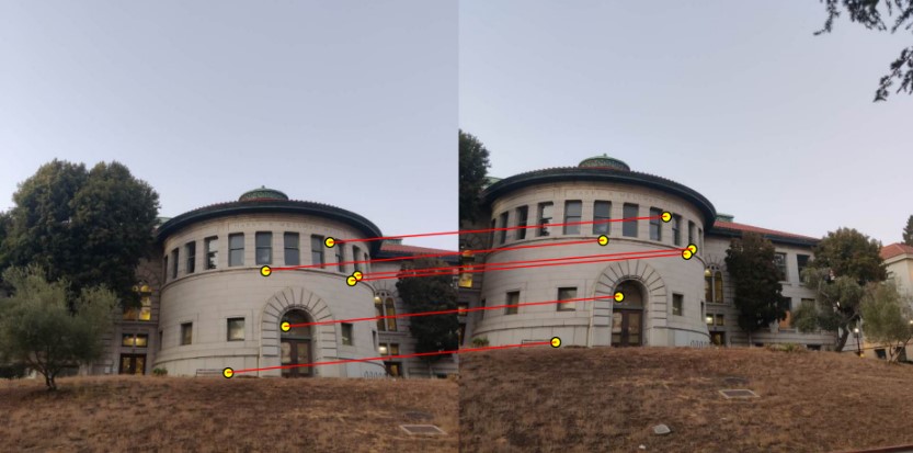
4-point RANSAC
Once we have the matching points, we can use RANSAC to caculate the homography matrix.
Firstly, we randomly select 4 points from the matching points, and caculate the homography matrix.
Then we caculate the distance between the points in the second image and the points in the first image after warping.
If the distance is smaller than the threshold, we will add this point to the inliers.
Repeat this process for several times, and select the homography matrix with the most inliers.
Then use this best homography matrix to caculate distance for all the points, and select the points with the distance smaller than the threshold as the inliers.
Finally, we caculate the homography matrix using the inliers.
One thing to notice is that we need to normalize the points before caculating the homography matrix.
And I repeat the process for 1000 times, and select the homography matrix with the most inliers.
Base on the paper, I set the ratio = 0.5, and the distance threshold around 1.
Blend the images
After we get the homography matrix, we can warp the image using the function warpImage(img, H),
and blend the images together to get the final result.
Outputs