Project 2

Part 1: Fun with Filters

Part 1.1: Finite Difference Operator

Workflow

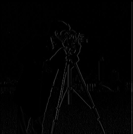
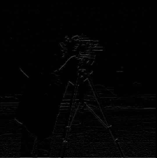
• First, we definded two array D_x ([1,-1]) and D_y ([1,-1].T), which are the finite difference operators in x and y direction.
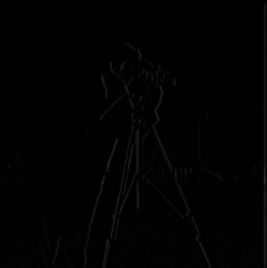
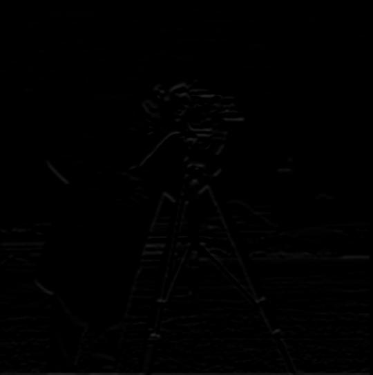
• Convolve the image by convolve2d function with these two arrays, to caculate the partial derivative in x and y direction.
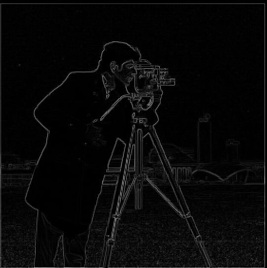
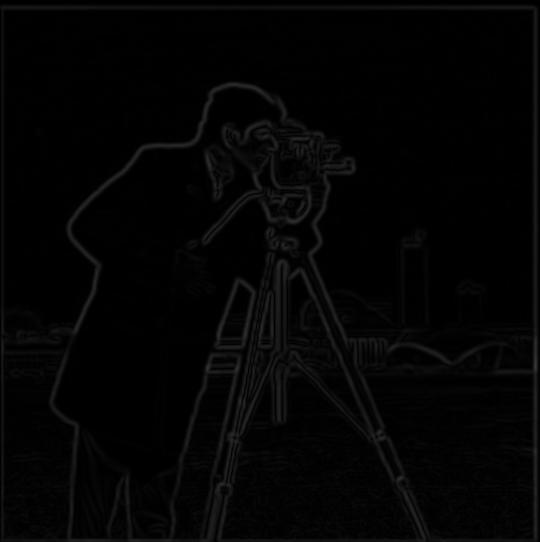
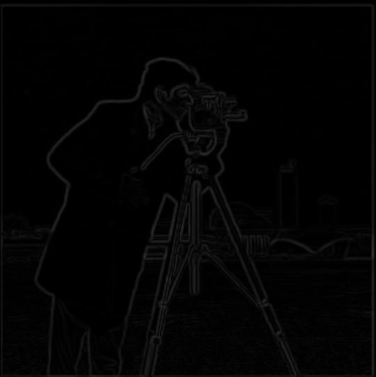
• After that, we use the formula: sqrt(dx^2 + dy^2) to caculate the gradient magnitude of the image. Gradient magnitude shows the change rate of the pixel value in x and y direction.
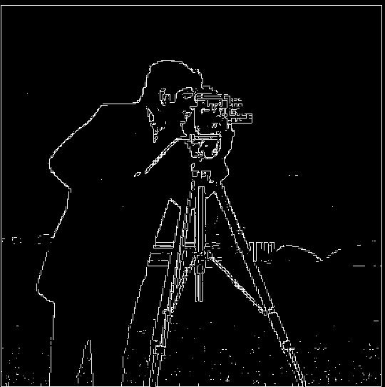
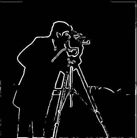
• However, there is some noise in the image, so we need to choice an appropriate threshold, convert the result to binary image.
• After trying, I found that the threshold 95.5% of the gradient magnitude is a good choice to get a clear binary image.

Results

Partial derivative X

Partial derivative y

P1_Magnitude

P1_binary

Part 1.2: Derivative of Gaussian (DoG) Filter

Reason

From Part1.2, we see the difference operator results has a lot noise, to reduce it we have to find appropriate threshold and then binary it. Derivative of Gaussian filter is mush smoother

Workflow

• To get a Gaussian filter, we first create a 1D Gaussian filter use cv2.getGaussianKernel function. Then take the outer product of the 1D Gaussian filter to get a 2D Gaussian filter.
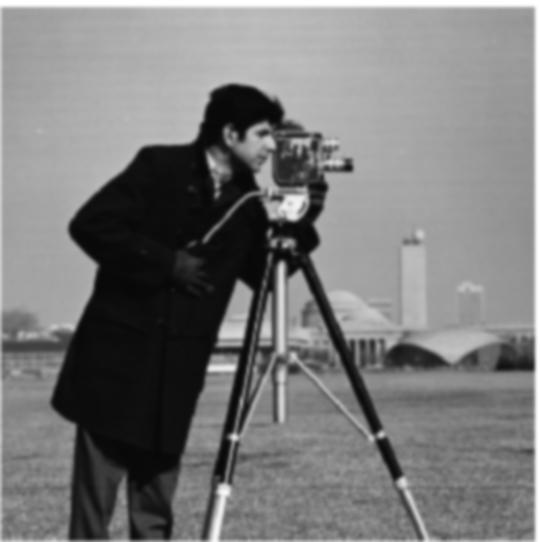
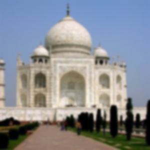
• With the Gaussian filter, we can create a blurred version of the original image by convolving the image with the Gaussian filter.
• After that, the same step as Part 1.1, we caculate the partial derivative in x and y direction, and then caculate the gradient magnitude of the image.

Here is some of the resulte and blurred image:

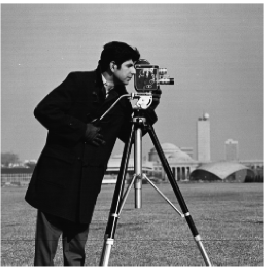
Original Image

Blurred Image

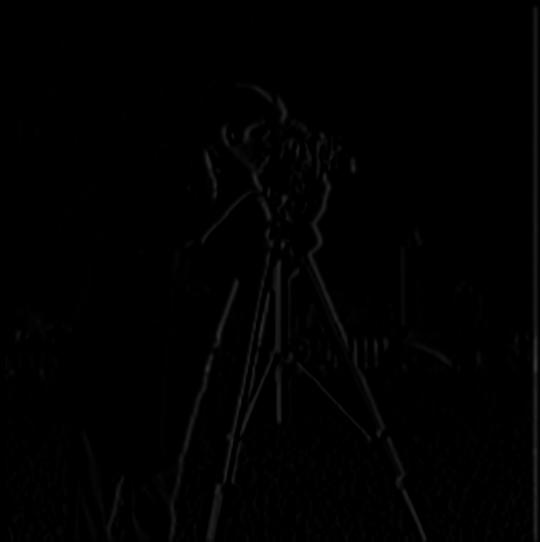
Partial derivative X

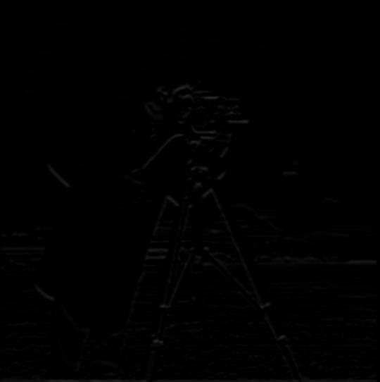
Partial derivative y

P2_Magnitude

P2_binary

To make the code faster, we can do the same thing as Part 1.2, but instead of convolving the image with the Gaussian filter and then convolving the result with the difference operator, we can first convolve the Gaussian filter with dx and dy, and then convolve the result with the image. This way, we only need to convolve the image once.
Below is the image of the result of this method:

P2_2_Partial derivative X

P2_2_Partial derivative y

P2_2_Magnitude

P2_2_binary

Part 2: Fun with Frequencies

Part 2.1: Image "Sharpening"

Workflow

• We use the Gaussian filter(Only pass low frequency) to blur the image, like what we did in Part 1.2.
• Then, we subtract the blurred image from the original image, which is the high frequency components of the image.
• After that, we can share the original image by adding the high frequency components times alpha to the original image.
  sharpened_image = original_image + alpha * high_frequency

Results

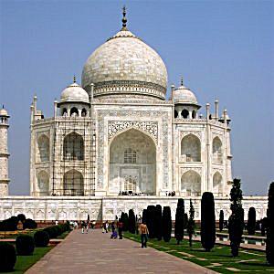
Original Image

Blurred Image

Sharpened Image(alpha = 1)

Original Image

Sharpened Image(alpha = 3)

Original Image

Blurred Image

Sharpened Image

Part 2.2: Hybrid Images

Hybrid images combining the low frequency components of one image with the high frequency components of another image. The image looks like the low frequency image, when we are far away, but when viewed up close, the image looks like the high frequency image.

Workflow

• First, use the provided code align_image_code.py to align the two images. Trying to find the best alignment of the two images.
• Try to find the best high and low frequency cutoff(sigma) of the two images. Repeat the step until find appropriate sigmas.
• Using the Gaussian filter to blur the first image, and then subtract the blurred image from the original image to get the high frequency components of the first image.
• Use the Gaussian filter to blur the second image, to get the low frequency components of the second image.
• We combine the low frequency components of the first image with the high frequency components of the second image to get the hybrid image by the

Results


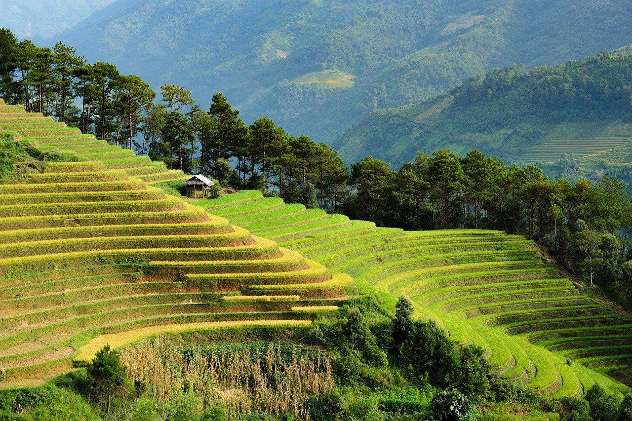
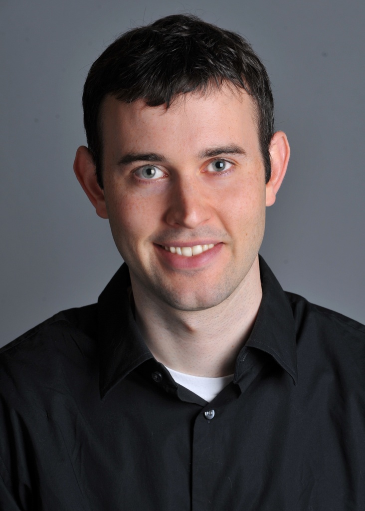
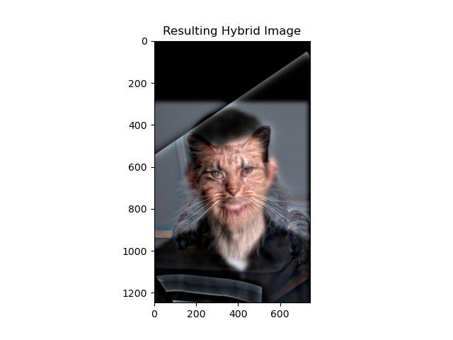
DerekPicture Image

nutmeg Image

Hybrid Image

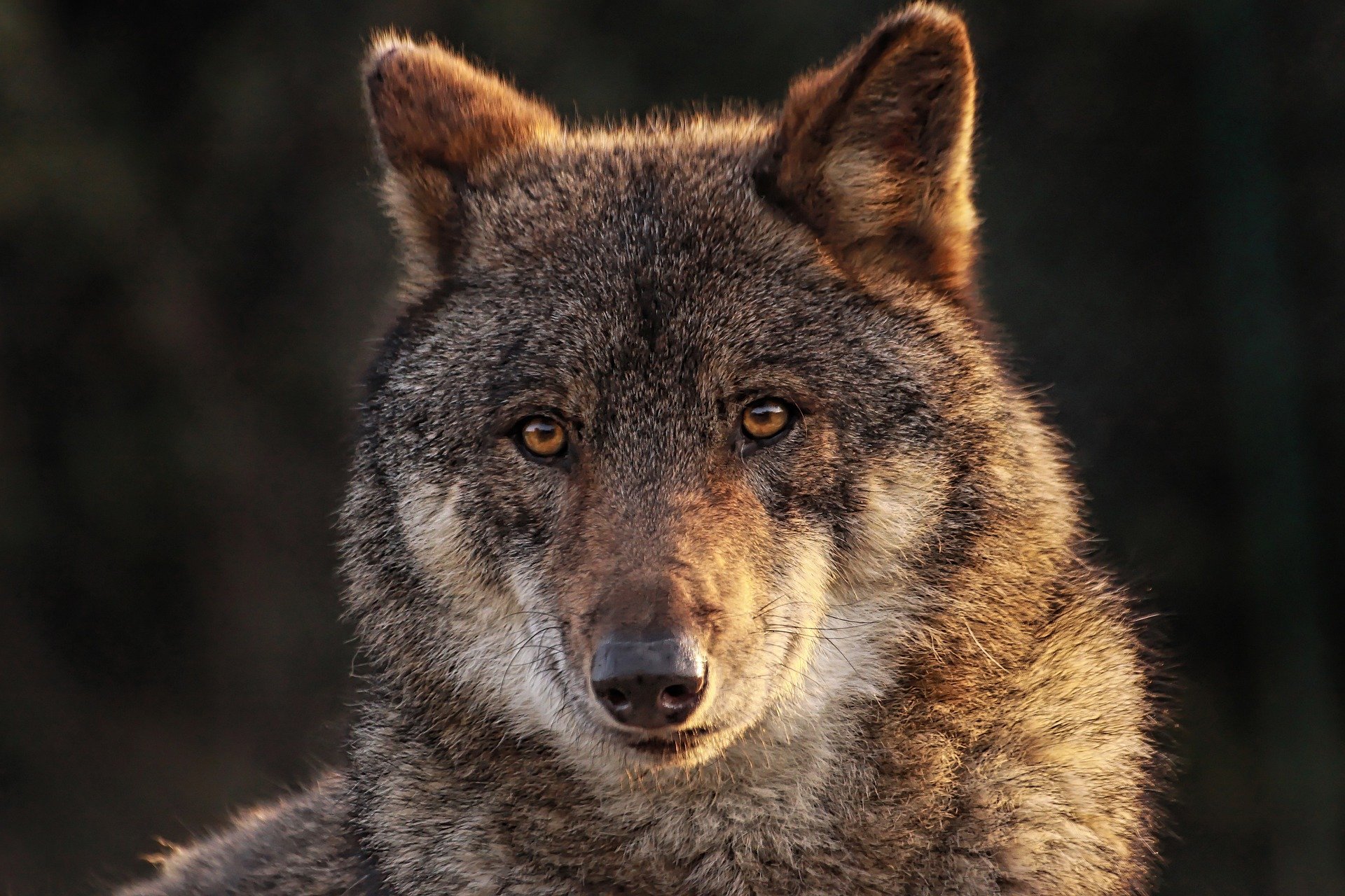
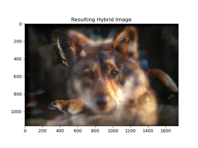
Wolf Image_low

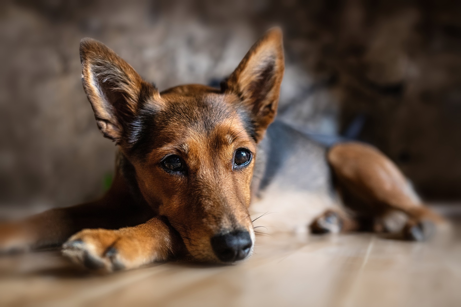
Dog Image_high

Hybrid Image

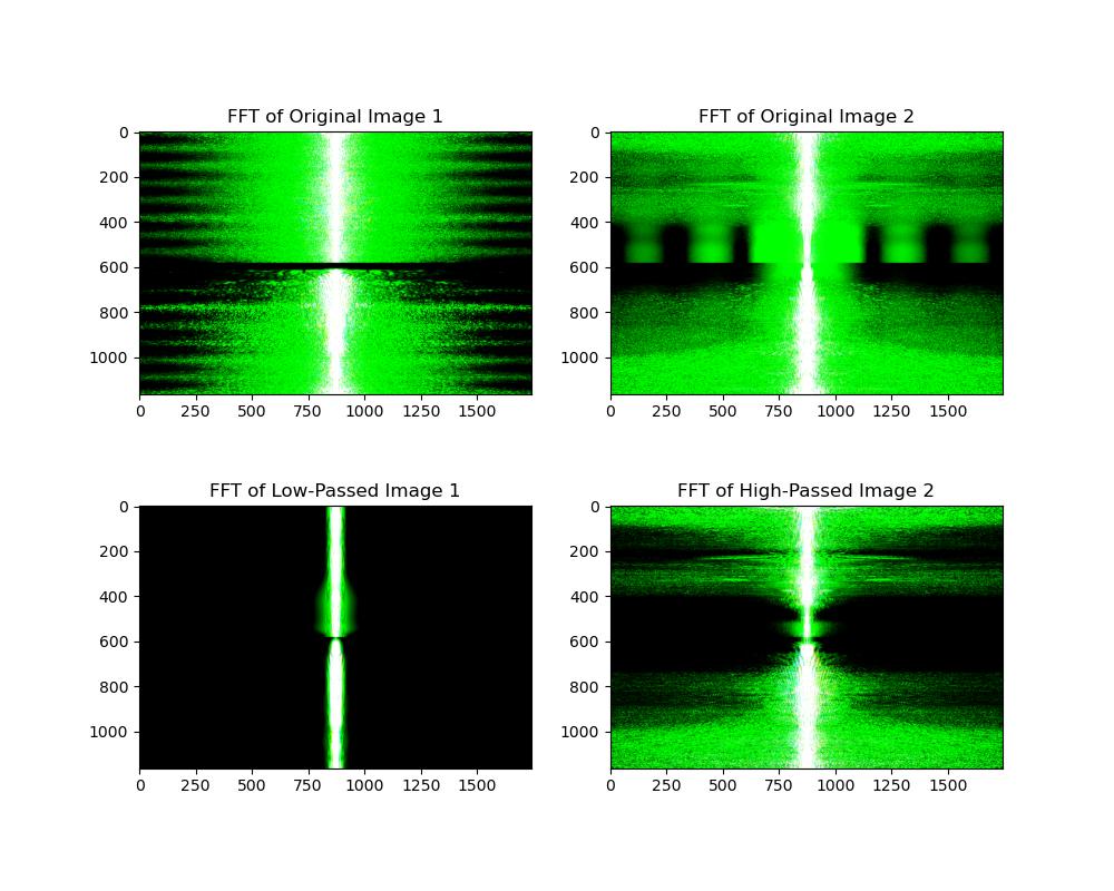
FFT Dog and Wolf Image

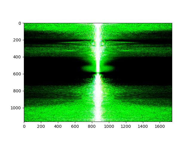
FFT Combined Image
From FFT images, we can see how the frequency components of the two images changed after apply high and low pass filter, and how they are combined. The low frequency components of the wolf image are combined with the high frequency components of the dog image. This two filtered images has a lot different frequency components, so the hybrid image looks like a wolf when we are far away, but looks like a dog when we are close.

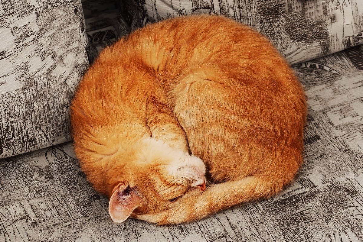
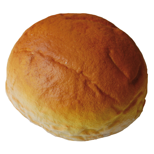
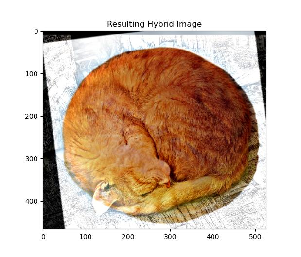
Cat Image_high

Bread Image_low

Hybrid Image

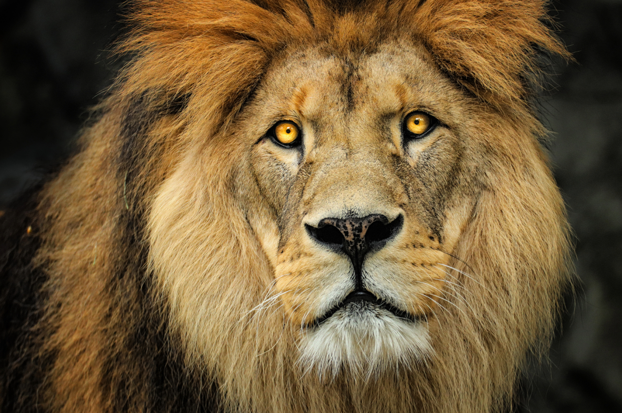
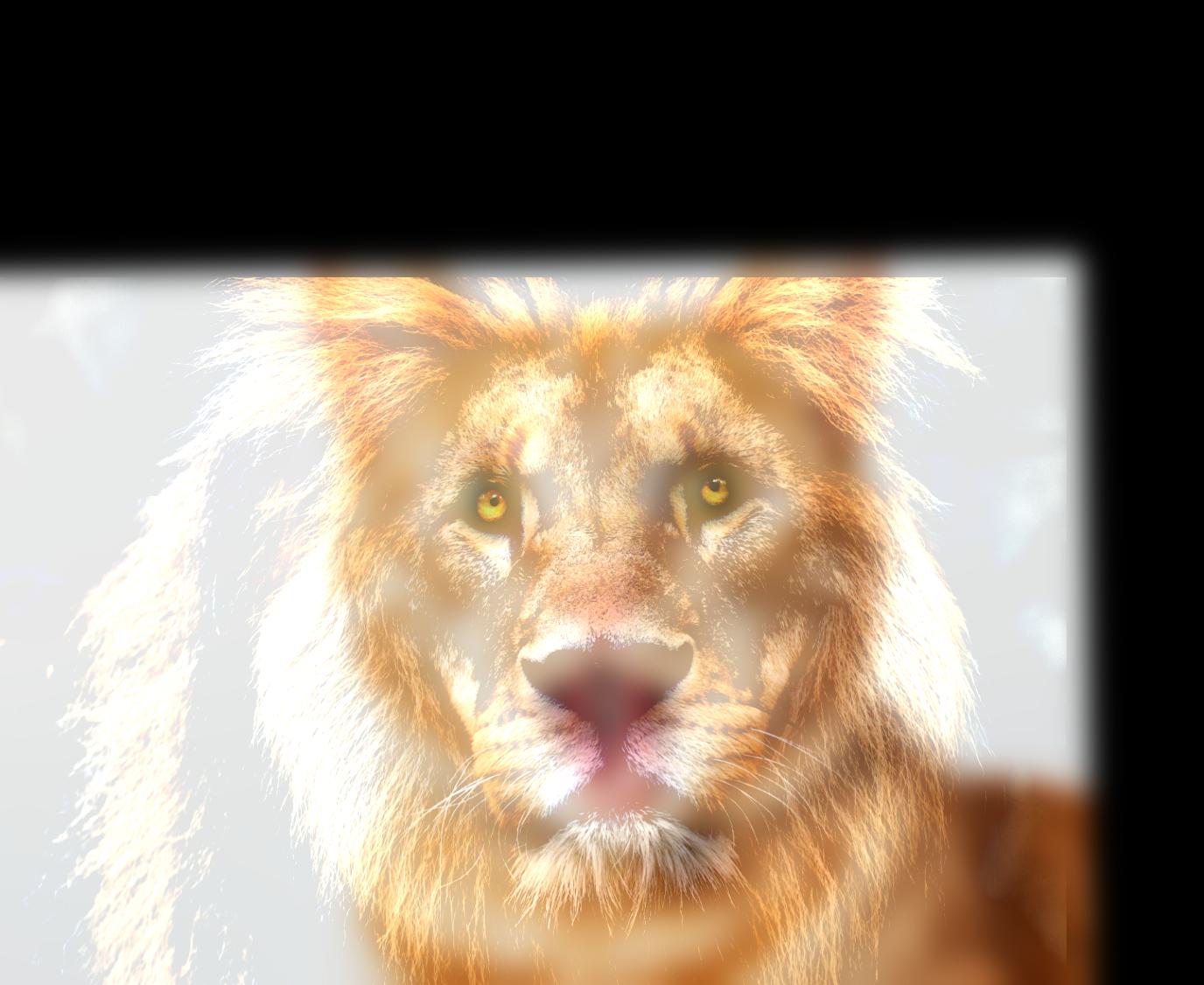
Lion Image

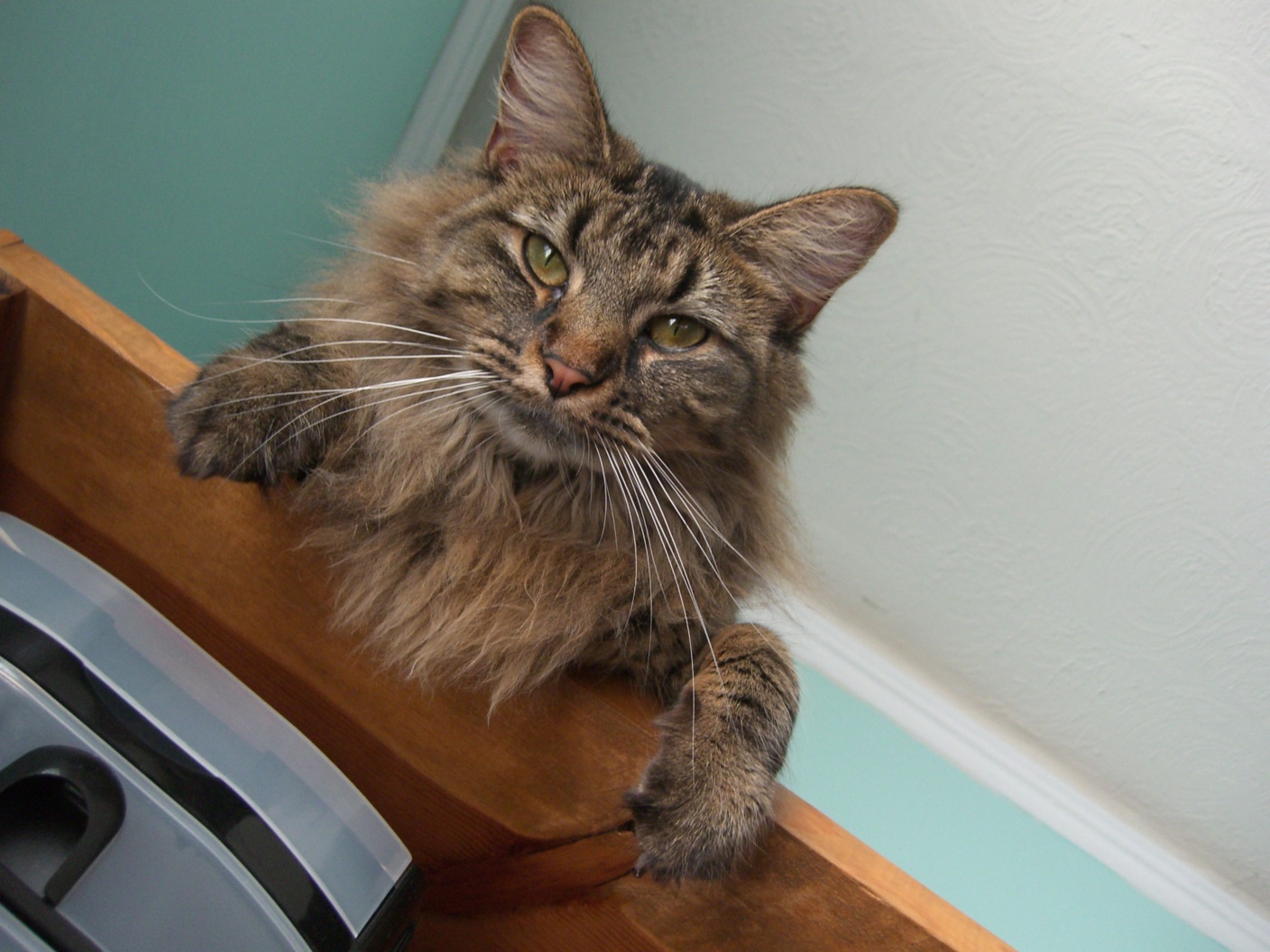
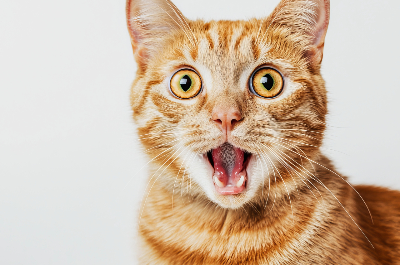
Cat Image

Bad Hybrid Image

Multi-resolution Blending and the Oraple journey

Overview:

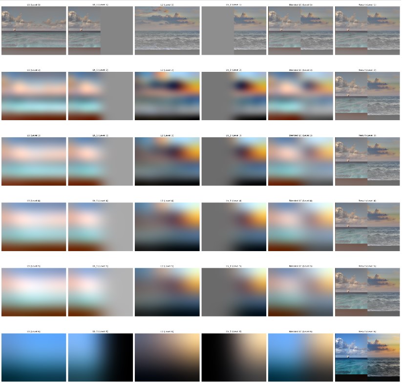
In this part, we are using Gaussian and Laplacian stacks to blend two images together.
The Gaussian stack (G = G.append(blur_im(im,filter))) is a series of images that are blurred with different sigmas, and the Laplacian stack (L = G[i] - G[i+1]) is the images that are the difference between the blurred image and the image to blurring To blend two images together, We blend the images together in each level of the two images Laplacian stack.

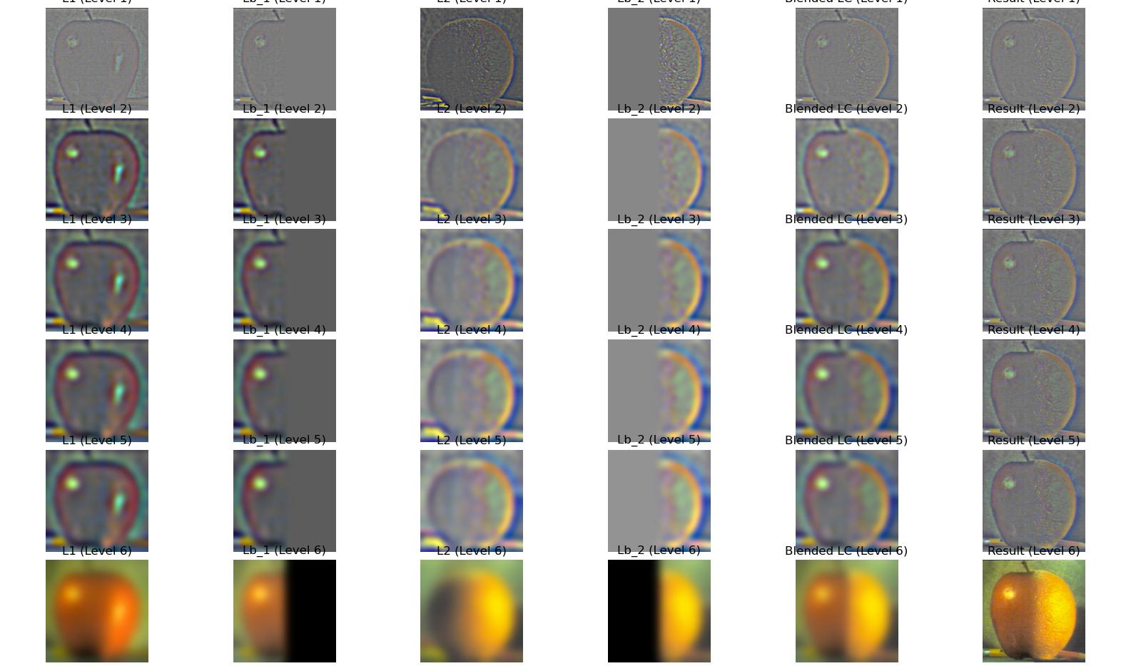
Part 2.3: Gaussian and Laplacian Stacks

Workflow

• Create the Gaussian stack and Laplacian stack of the two images.
• Then blend the images together in each level of the two images Laplacian stack, save the result in the blended stack.
• Finally, we add all of the images in the blended stack together to get the blended image.

Results



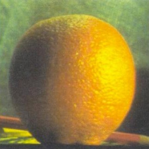
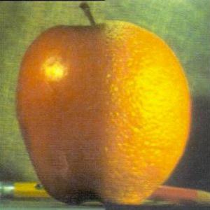
Orange Image

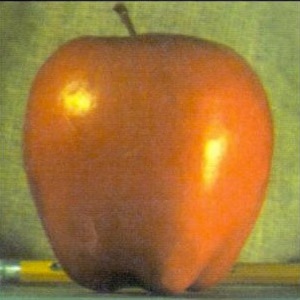
Apple Image

Blended Image

Part 2.4: Multiresolution Blending

Overview:

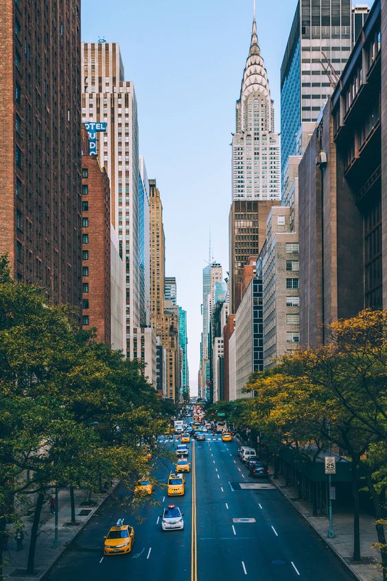
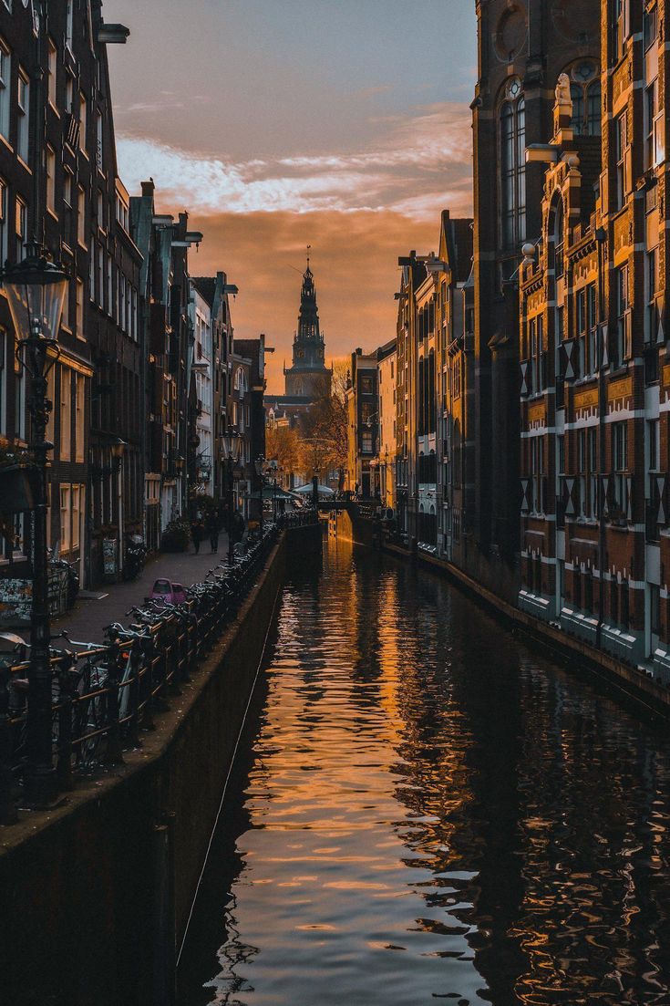
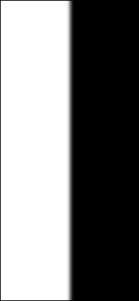
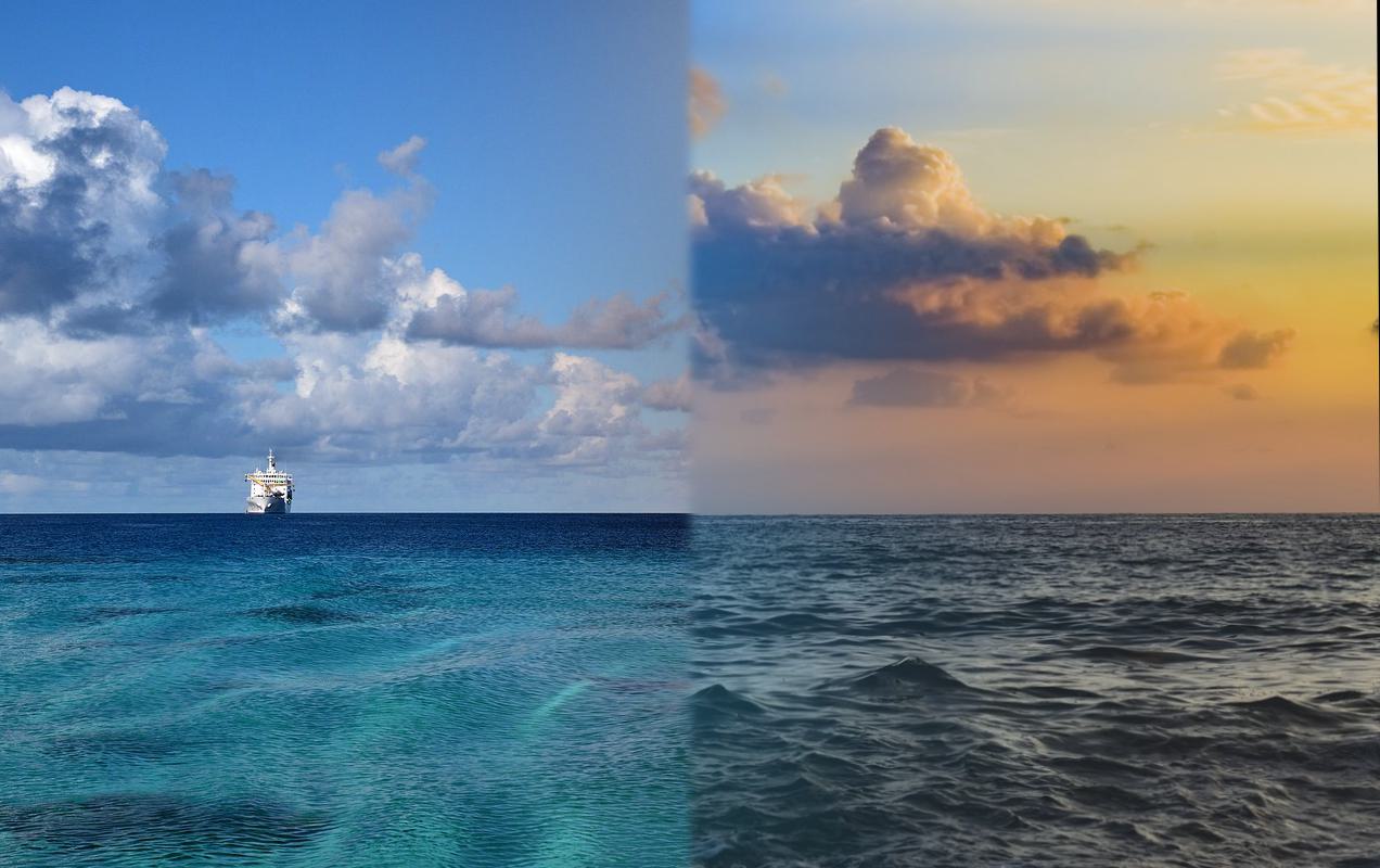
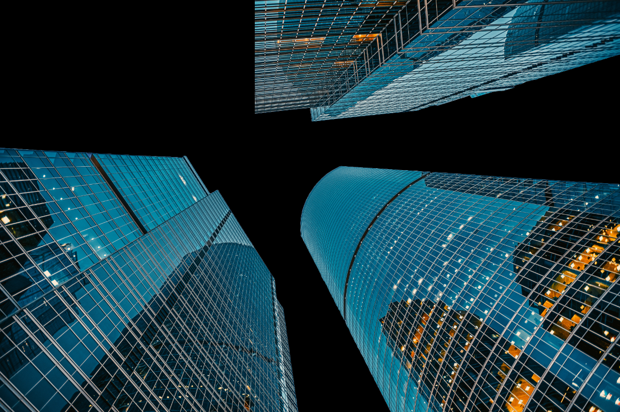
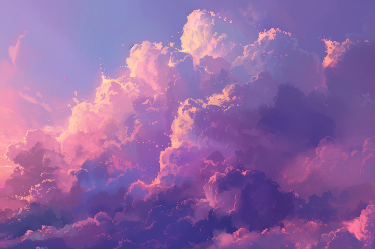
Using the function from last part, we can easily blend two images together. Add all levels blend images together, we can get the final result. For the irregular mask, I used adrobe express to create a mask, and then convert it to a binary image. All images provied by adrobe express are resized to the same size.

Output















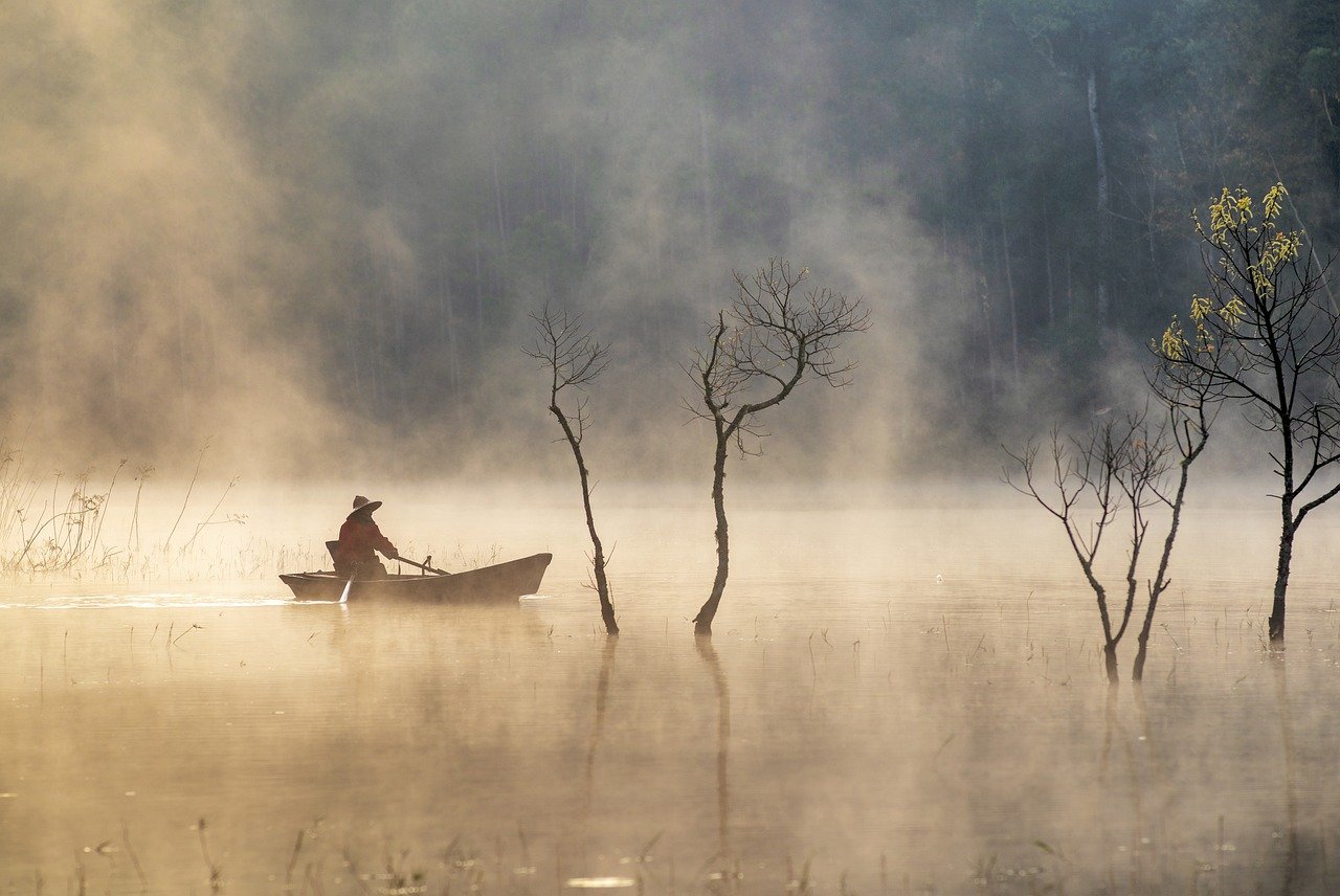
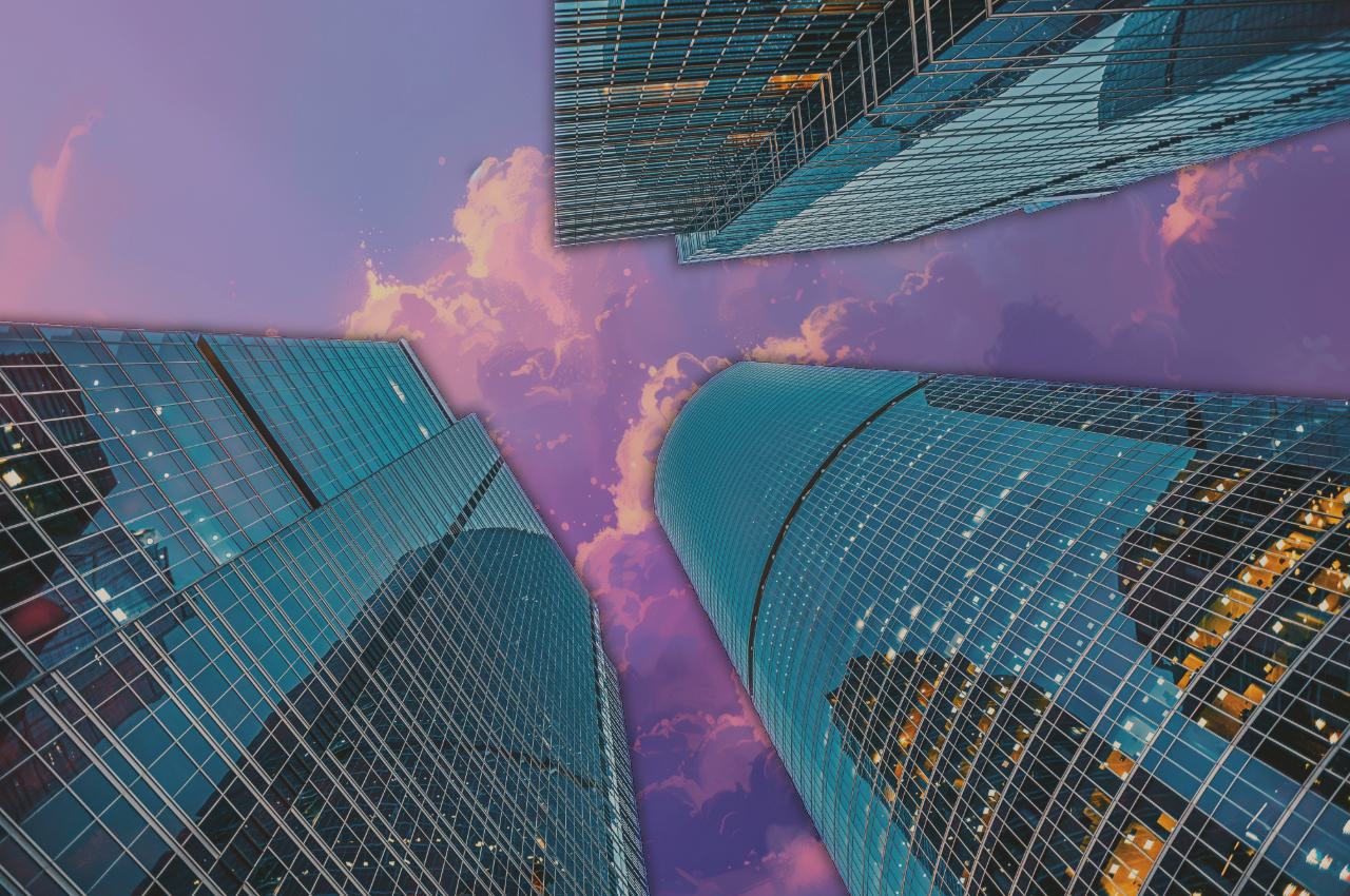
Image 1

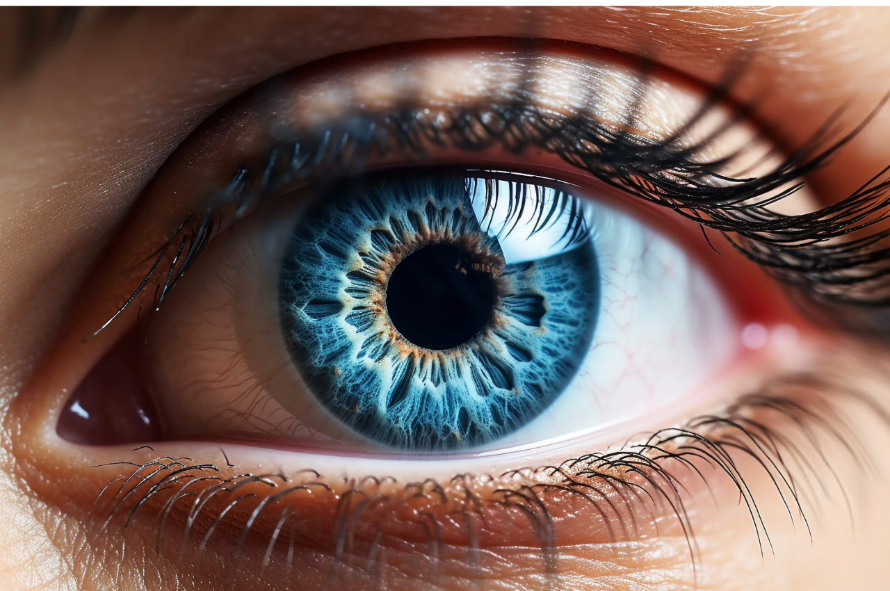
Image 2

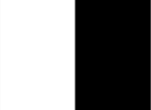
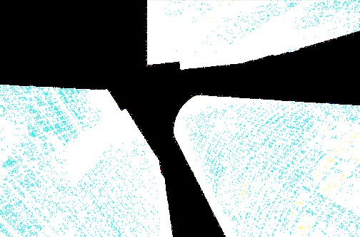
Mask

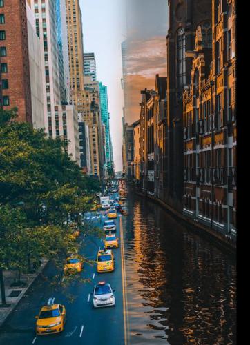
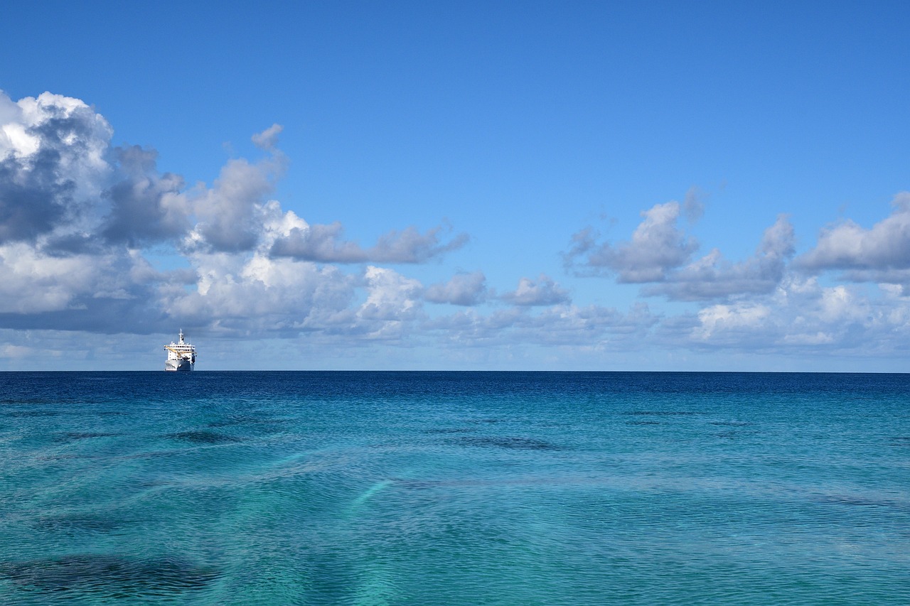
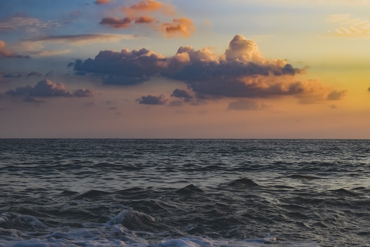
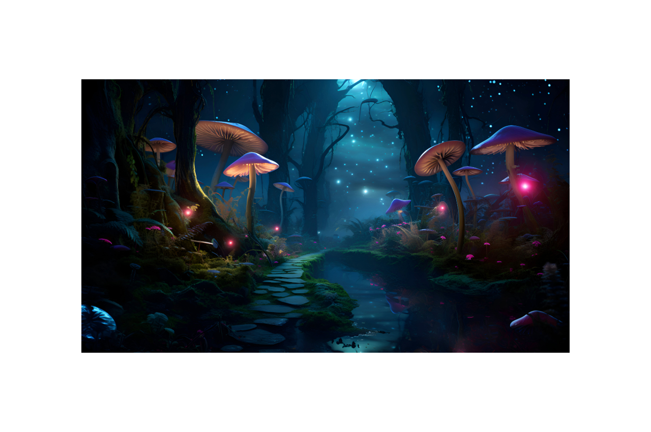
Blended Image